Eight business questions, eight filters
Each story starts with a question asked in a technical department, a local authority or a consultancy, then translates it into FilterMate settings, step by step, on the complete BD TOPO of a French department. The screenshots show the whole QGIS window so you can compare with your own screen, and every result comes with its numbers.
The commune dossier in three minutes
Scope 12 department-wide layers to one commune and deliver a GeoPackage with project and styles.
PlanningWho lives next to the main roads?
A buffer computed by expression from the road importance, for noise classification.
RiskHow far the Garonne can reach
A 300 m then 100 m band around water surfaces, undo and replay.
StructuresEvery bridge in the metropolis
Scope on a 37-commune EPCI, then the Cross predicate between roads and watercourses.
ForestryClearing brush around homes
Expression selection, 50 m buffer, a second attribute filter chained with AND.
RescueHamlets the rescue services reach badly
The Disjoint predicate: whatever lies more than 200 m from a paved road.
TeamThe query library
Save a filter as a favorite, replay it, describe it, share it.
GIS administrationWhat changed?
The Processing batch filter on four layers and 1.6 million objects.
0The playground
Every story uses the same file: the BD TOPO 3.5 of Haute-Garonne, exactly as the French mapping agency (IGN) distributes it for free on the Géoplateforme, in a single 2.9 GB GeoPackage with 53 layers. Nothing was clipped beforehand: FilterMate scopes the territory every time.
| Layer | Features in the department | Role in the stories |
|---|---|---|
batiment (buildings) | 1,173,829 | Main target: what is protected, what is served |
troncon_de_route (road segments) | 383,112 | Source of road buffers, target of crossings |
haie · zone_de_vegetation (hedges, vegetation) | 416,105 · 261,051 | Vegetation to clear |
troncon_hydrographique · surface_hydrographique | 49,344 · 9,969 | Watercourses and water surfaces |
erp (public buildings) | 11,384 | Schools, town halls, shops |
construction_lineaire | 12,473 | Bridges, dams, walls |
commune · epci | 930 · 38 | Scoping territories |
filtermate.log on an ordinary laptop.
1The commune dossier in three minutes
The need
Camille, a project officer in a consultancy, is answering a tender from the town of Saint-Gaudens. She has the complete department GeoPackage and must deliver tonight only what concerns the commune: buildings, roads, hydrography, vegetation, facilities. With styles, in a file the client opens with a double-click.
The FilterMate translation
The commune is the source layer, picked by name in single selection. Every other layer is ticked at once in Layers to filter, with the Intersect predicate and no buffer. The Exporting tab then writes a GeoPackage with embedded project, QML styles and a ZIP archive.
- Load the 13 layers and open FilterMate. The Layers panel shows the counts of the whole department: 1,173,829 buildings, 383,112 road segments. Click commune: it becomes the source layer. In the Exploring area, tick Single selection, set the display expression to
"nom_officiel"and type "Saint-Gaudens" in the list. The Tracking button of the Exploring column being on, the canvas recentres on the commune by itself.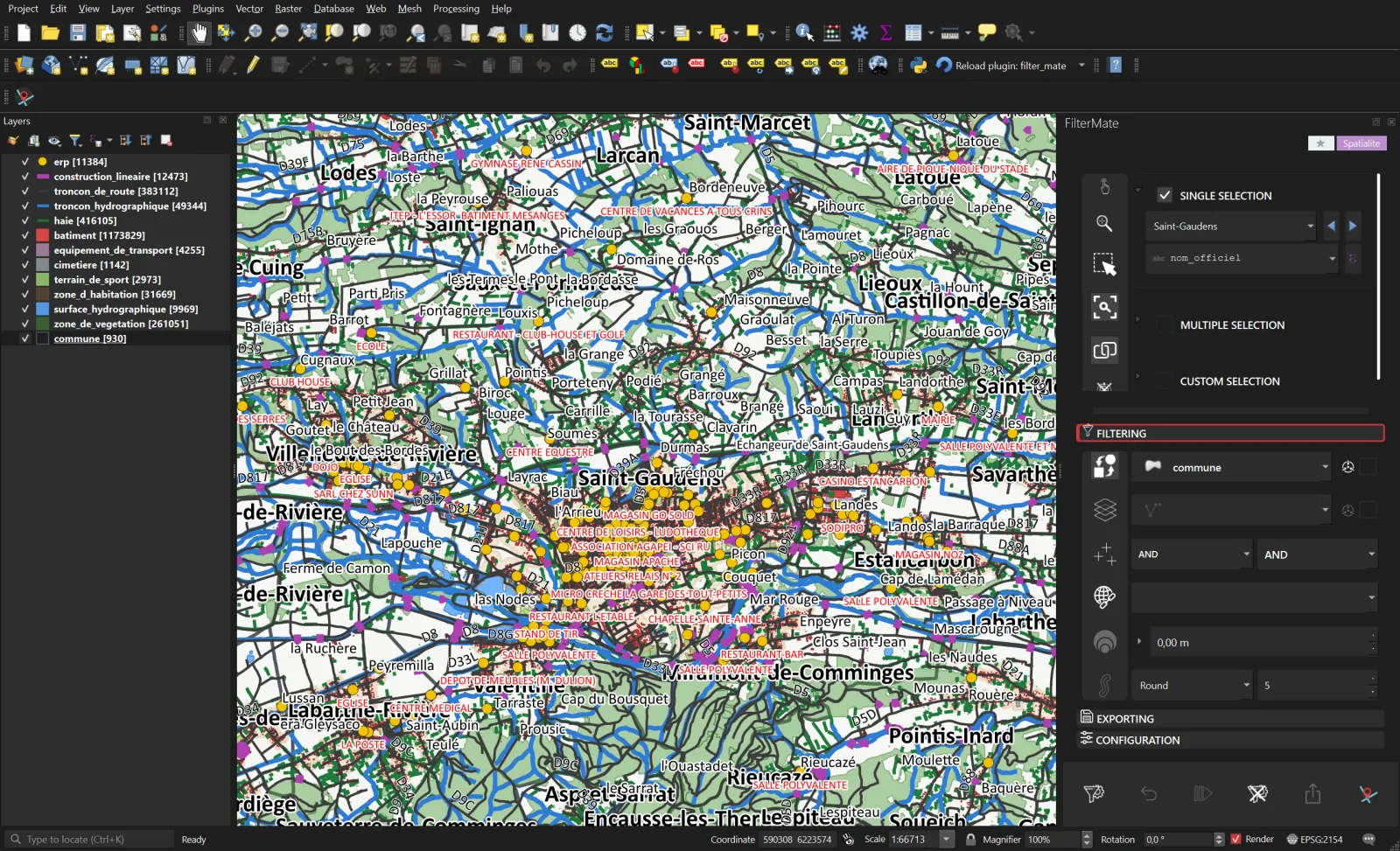
Step 1. The commune is selected (yellow highlight); around it the whole department is still loaded. - Tick every target. Filtering tab, Layers to filter row: right-click in the list, then Select All. The Intersect predicate is ticked, the Buffer row stays off.
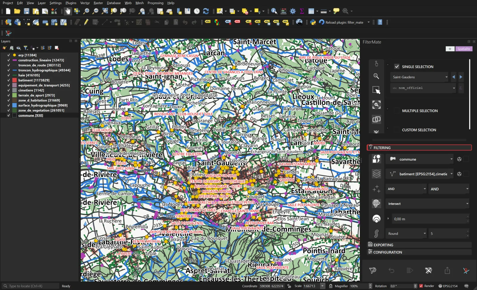
Step 2. Twelve target layers, one predicate, no buffer. - Filter. The log reports under a second for the twelve layers: on GeoPackage, FilterMate first queries the R-tree index of each table, then evaluates
ST_Intersectson the candidates only.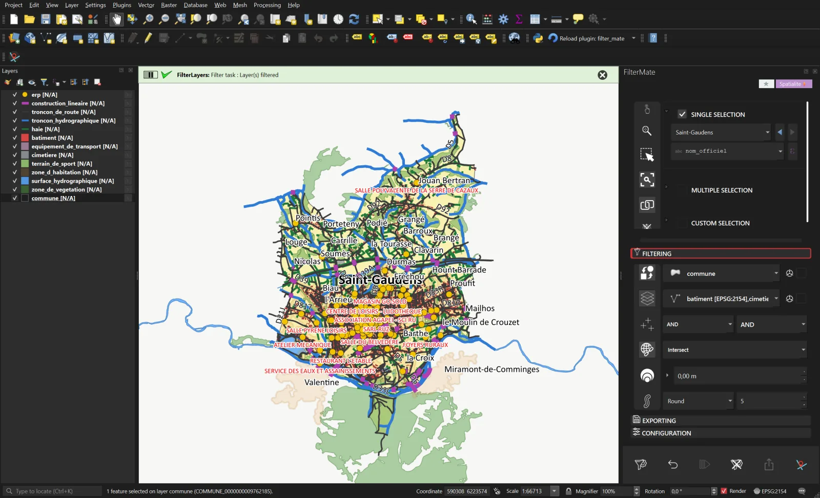
Step 3. The layers only show the commune's content. Vegetation polygons straddling the boundary are kept whole: that is what Intersect means. 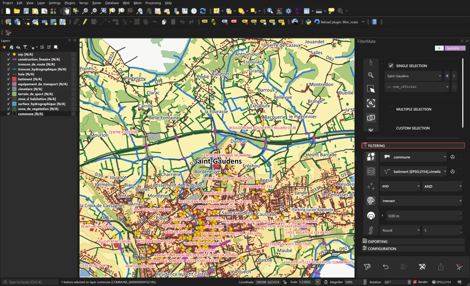
Zoom on the town centre: 12,380 buildings, 317 public buildings, 2,902 road segments. - Configure the export. Exporting tab: the 12 layers, EPSG:2154, styles as QML, GPKG format, output folder and a ZIP archive.
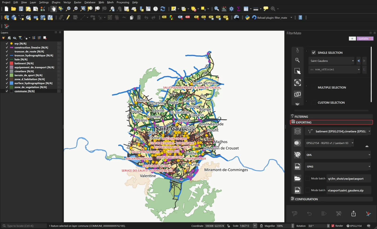
Step 4. Everything is set, nothing is written yet. - Export. Because the format is GeoPackage and several layers are exported, FilterMate shows a recap and offers to keep the group hierarchy. Confirm: the file is written in 4 seconds with an embedded QGIS project.
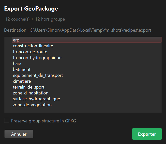
The recap before writing. 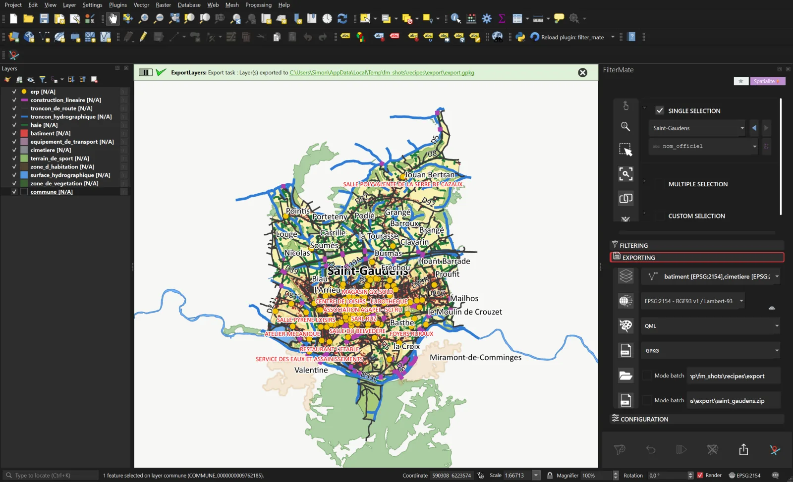
Step 5. Export done; the client will open the .gpkg and find the map as is.
Result
| Layer | Department | Saint-Gaudens |
|---|---|---|
| batiment | 1,173,829 | 12,380 |
| troncon_de_route | 383,112 | 2,902 |
| haie | 416,105 | 1,505 |
| zone_de_vegetation | 261,051 | 1,006 |
| erp | 11,384 | 317 |
| troncon_hydrographique | 49,344 | 157 |
| zone_d_habitation | 31,669 | 109 |
| construction_lineaire | 12,473 | 77 |
| surface_hydrographique | 9,969 | 42 |
| equipement_de_transport | 4,255 | 39 |
| terrain_de_sport | 2,973 | 27 |
| cimetiere | 1,142 | 2 |
Under the hood
Provider filter generated for the buildings layer, as read in Layer Properties → Source:
ROWID IN (SELECT id FROM "rtree_batiment_geometrie"
          WHERE minx <= 517706.0 AND maxx >= 511938.3
            AND miny <= 6231762.5 AND maxy >= 6222765.8)
AND ST_Intersects("geometrie", ST_MakeValid(ST_GeomFromText('Polygon ((…))', 2154)))2Who lives next to the main roads?
The need
Nadia is writing the noise chapter of the local plan of Muret, crossed by the A64 motorway and several departmental roads. The noise classification of infrastructures imposes sector widths that depend on the road category. She wants the list of buildings and public buildings located in those sectors, with a width that depends on each road.
The FilterMate translation
After scoping on Muret, the source layer becomes troncon_de_route with the custom selection "importance" IN ('1', '2'). The buffer is an expression evaluated for each segment: 300 m for importance 1, 250 m for importance 2. The Flat buffer type avoids round ends at segment tips. Targets: batiment and erp.
- Scope Muret. Same gesture as in story 1: commune as source, Muret in single selection, every layer as target, Intersect, Filter. Muret has 19,458 buildings, 354 public buildings and 5,512 road segments.
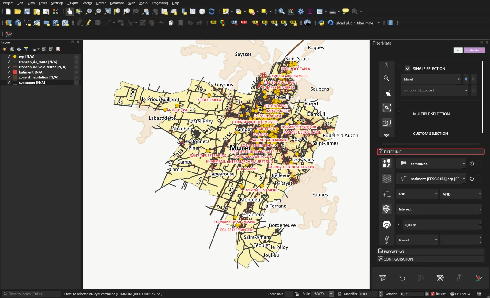
Step 1. The commune is scoped; the A64 crosses it from north-east to south-west. - Pick the main roads. Click troncon_de_route in the Layers panel: it becomes the source. Tick Custom selection and type
"importance" IN ('1', '2'). 102 segments are kept out of the commune's 5,512.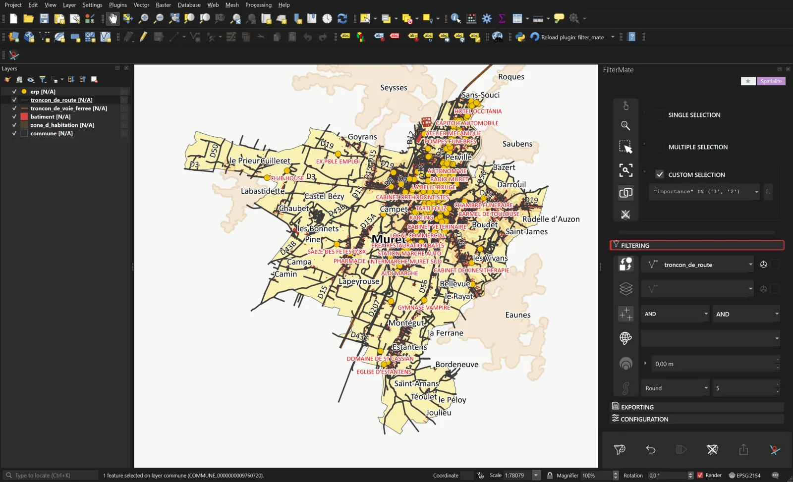
Step 2. The motorway and the main departmental roads are highlighted. - Buffer by expression. Targets batiment and erp, Intersect predicate. On the Buffer value row, click the small arrow left of the field to switch to expression mode and type:
On the next row, choose the Flat type.CASE WHEN "importance" = '1' THEN 300 WHEN "importance" = '2' THEN 250 ELSE 100 END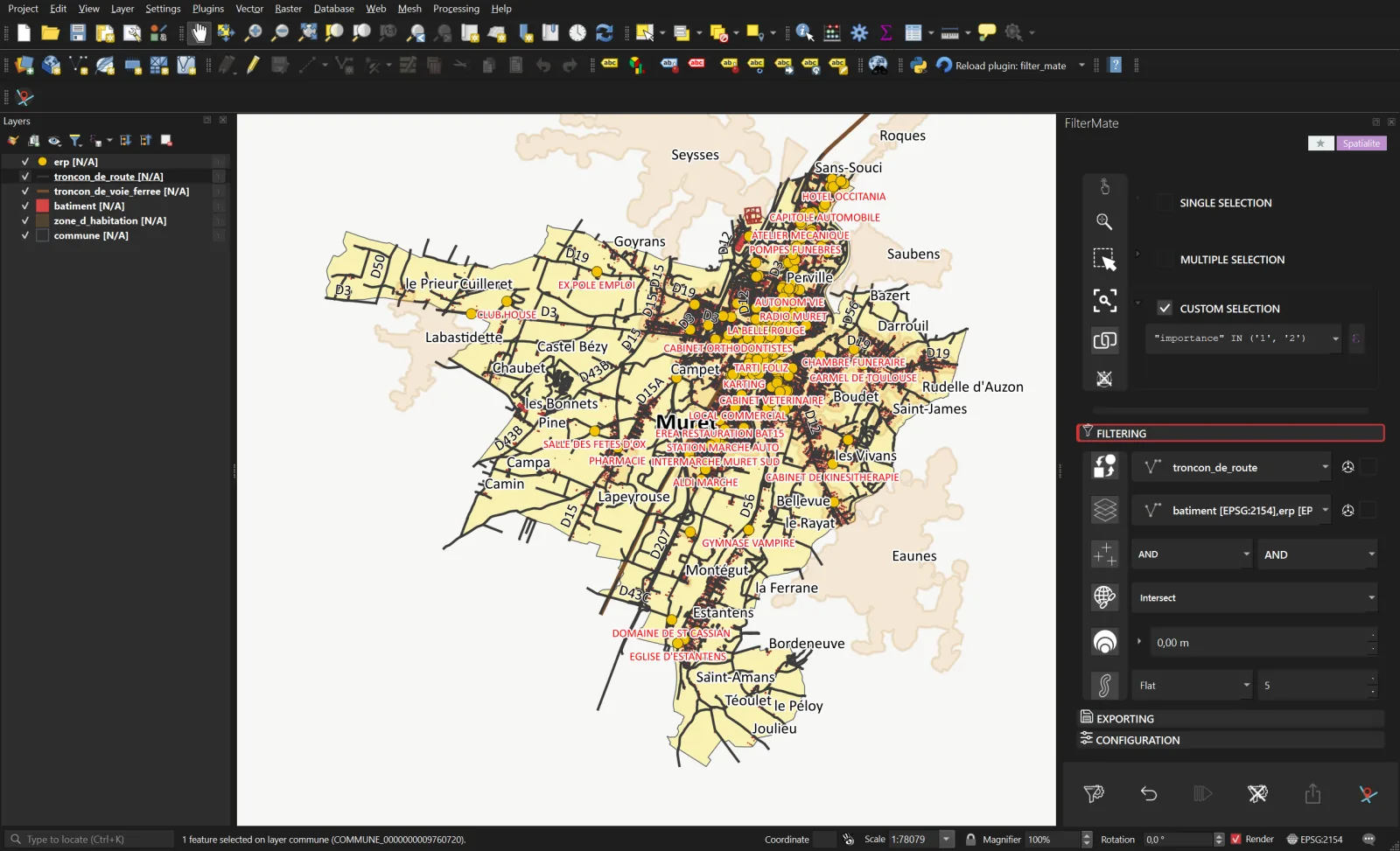
Step 3. The distance is no longer a number but a QGIS expression evaluated segment by segment. - Filter.
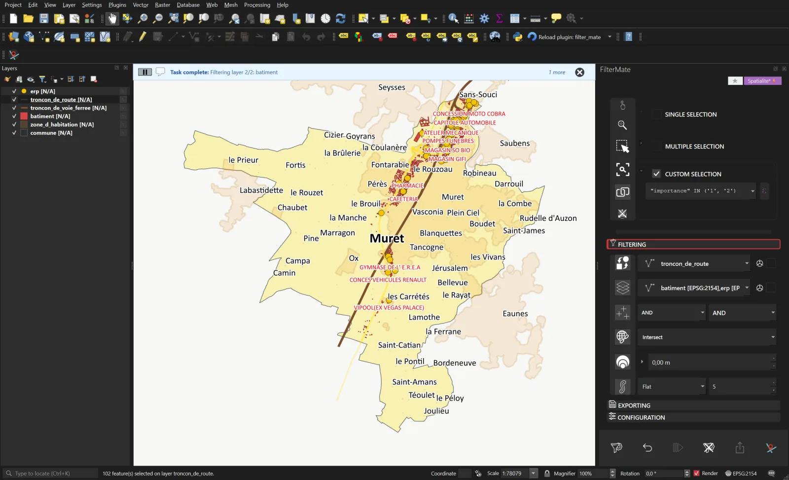
Step 4. Buildings and public buildings outside the sectors have left the map. 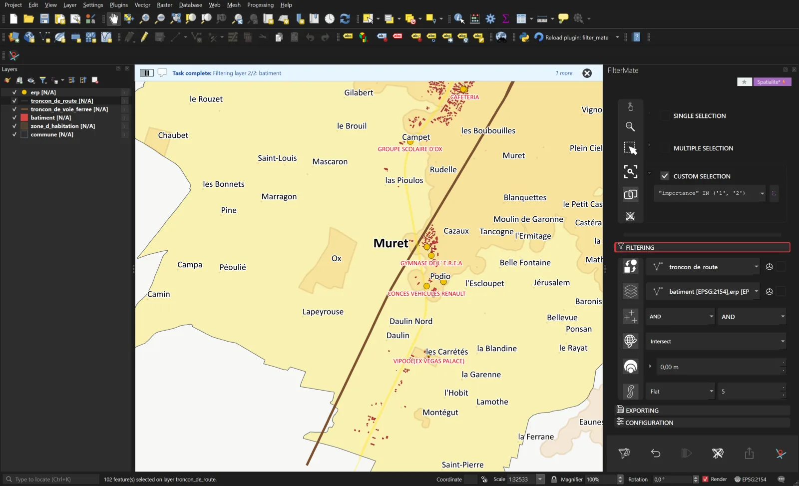
Zoom: the 300 m band around the A64 shows in the distribution of the remaining buildings.
Result
1,999 buildings and 74 public buildings of Muret lie in the noise sectors of the 102 segments of importance 1 and 2.
"largeur_de_chaussee" * 3.
Segments with an empty width need a coalesce("largeur_de_chaussee", 3).
3How far the Garonne can reach
The need
Julien prepares, for the planning department of Grenade, a meeting on the flood risk prevention plan. The commune sits at the confluence of the Garonne and the Save. He first wants to show everything within 300 m of the water surfaces, then tighten to 100 m for the frequent flood, and be able to step back in front of the councillors.
The FilterMate translation
Source: surface_hydrographique, scoped on Grenade, with a multiple selection and Select All (77 surfaces). Targets: buildings, public buildings and roads, Intersect predicate, 300 m buffer. A second Filter at 100 m, then Undo in the action bar.
- Scope Grenade. 6,998 buildings, 79 public buildings, 1,978 road segments and 77 water surfaces.
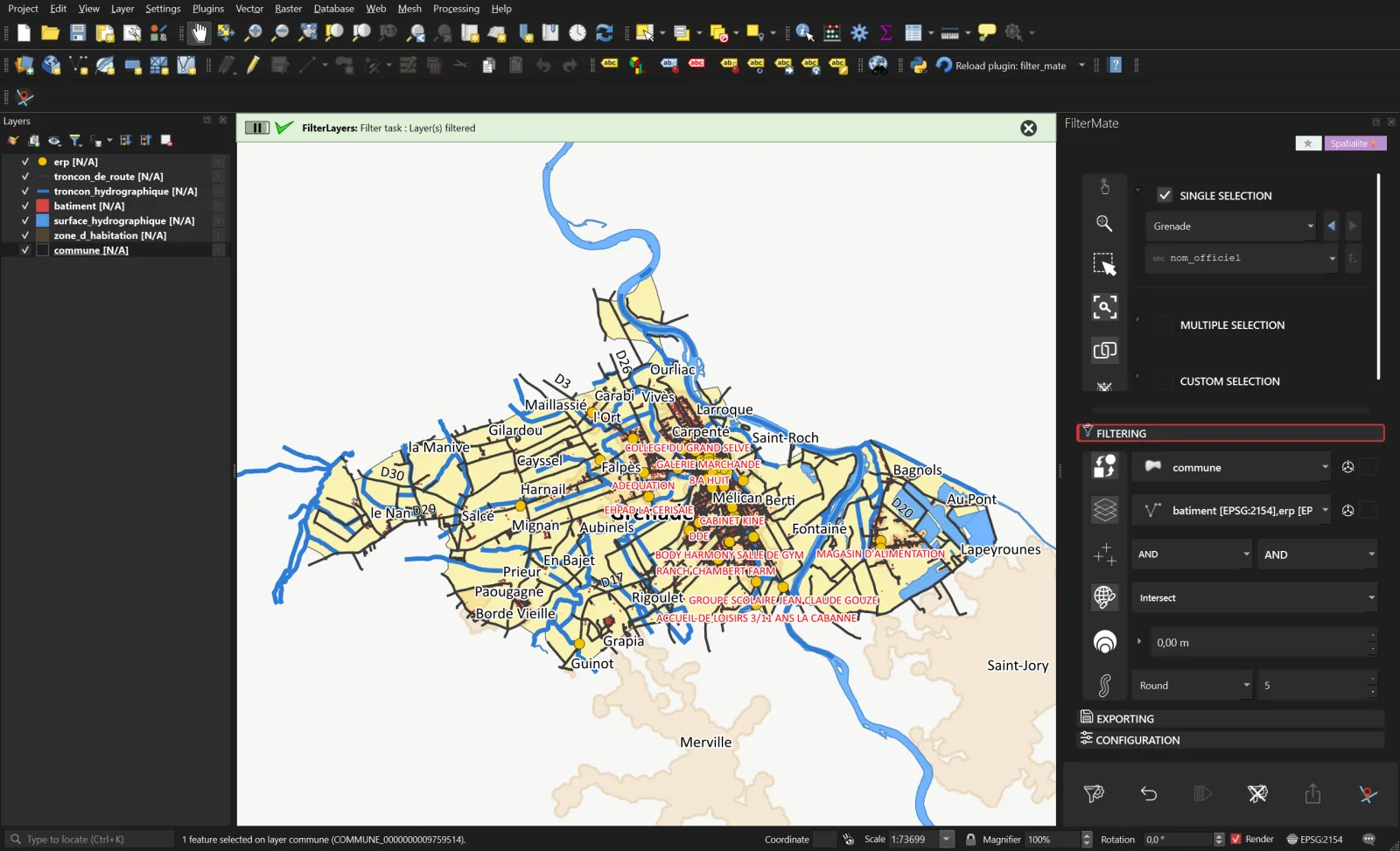
Step 1. The water surfaces (Garonne to the east, Save to the south) are now the only ones on the map. - Select every water surface. Click surface_hydrographique, tick Multiple selection, then right-click in the list and Select All. The summary above the list counts 77 features.
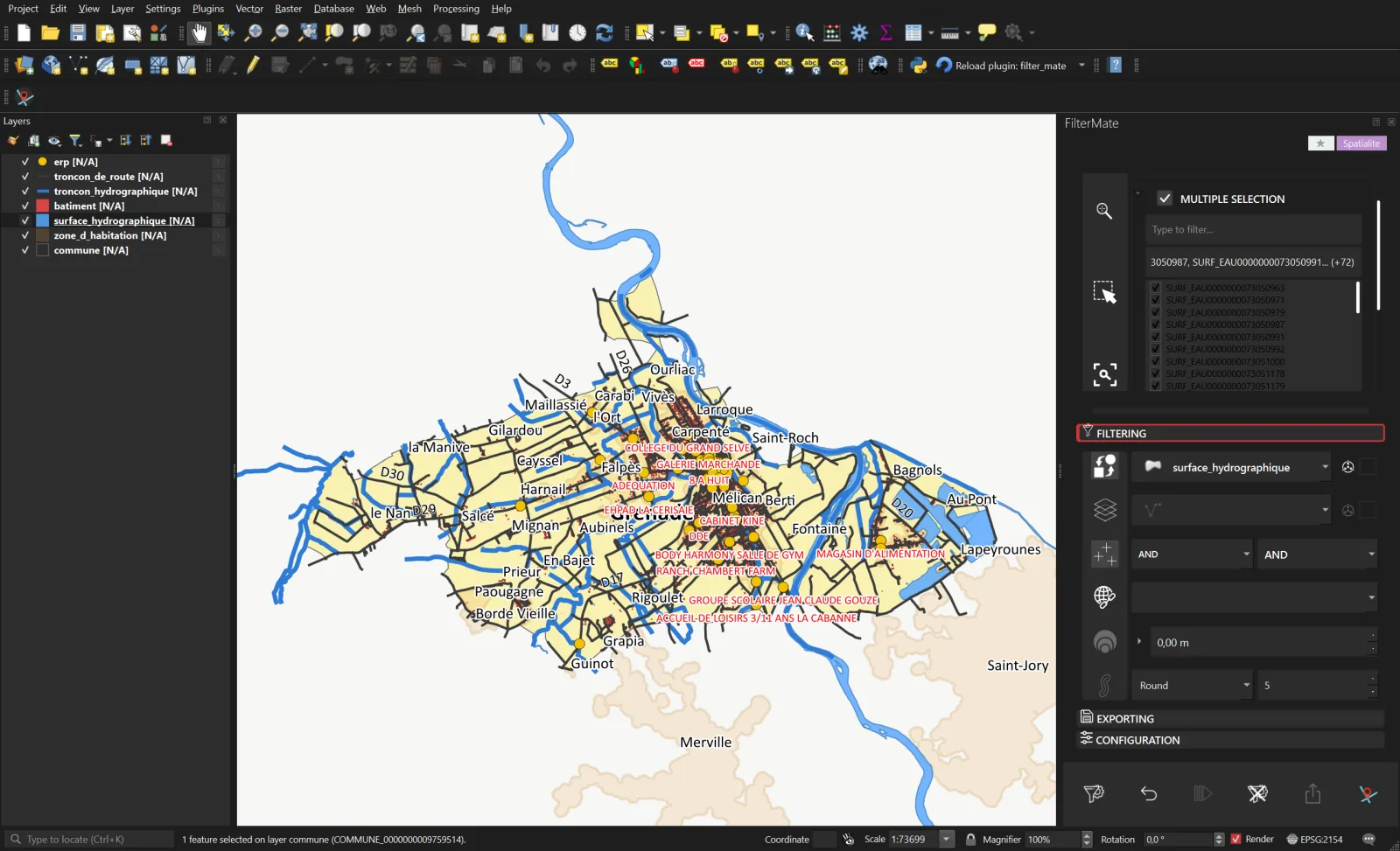
Step 2. The list shows the nature and id of each surface; all are ticked. - 300 m. Targets batiment, erp and troncon_de_route, Intersect, Buffer value 300. Filter.
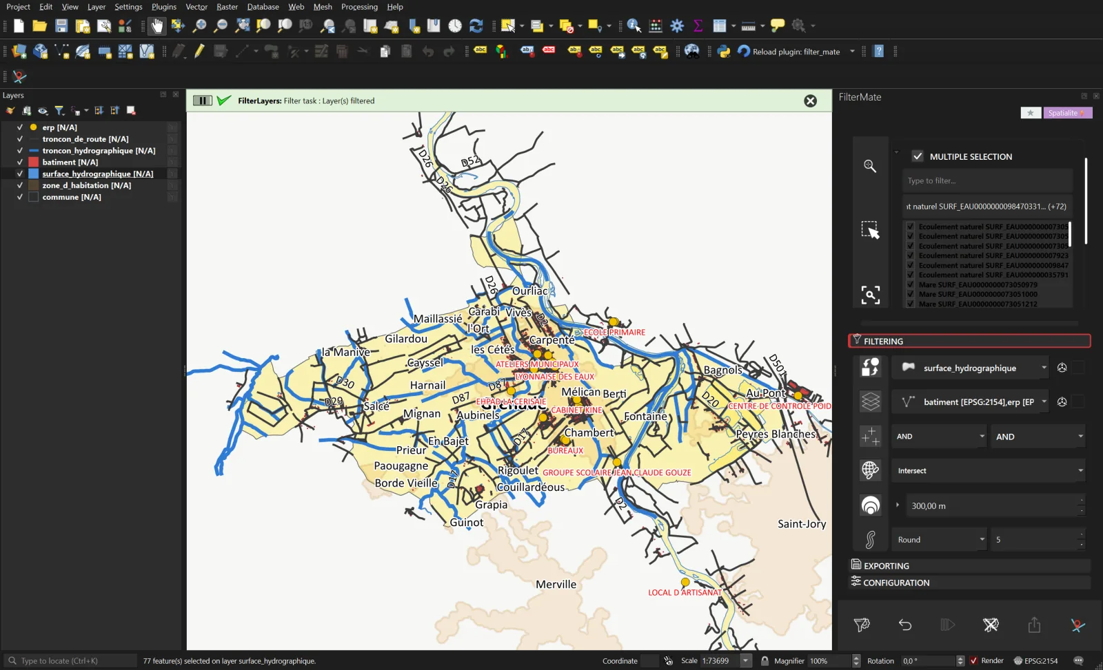
Step 3. The 300 m band follows the Garonne well beyond Grenade: the river polygons are long, and the targets' spatial filter replaces the commune scope. - 100 m. Change the buffer value and press Filter again.
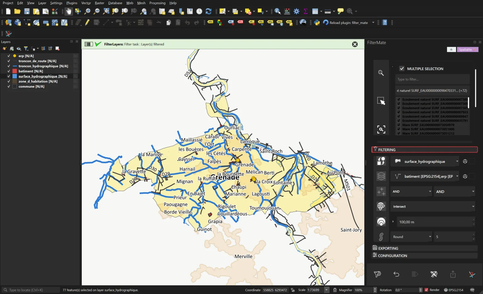
Step 4. The result tightens onto the banks. - Undo. The first button after Filter restores the previous state of the three layers, at 300 m. Redo would reapply it. The history belongs to the project and survives a QGIS restart.
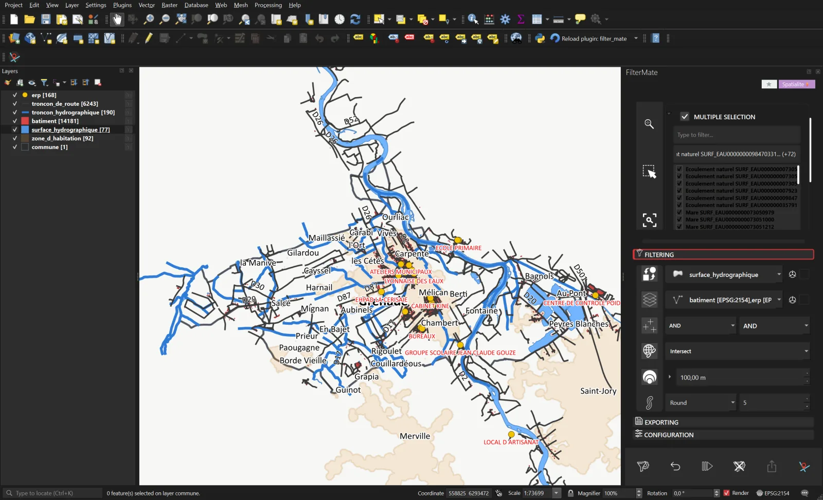
Step 5. Back to 300 m in one click.
Result
| Band | Buildings | Public buildings | Road segments |
|---|---|---|---|
| 300 m around Grenade's water surfaces | 14,181 | 168 | 6,243 |
| 100 m | 2,727 | 27 | 1,934 |
4Every bridge in the metropolis
The need
Karim manages the engineering structures of Toulouse Métropole: 37 communes, close to 99,000 road segments. He wants the inventory of the places where roads cross a permanent watercourse, segments and structures, to plan inspections.
The FilterMate translation
Scoping is done this time on the epci layer. Then the source becomes troncon_hydrographique with the custom selection "persistance" = 'Permanent', the targets troncon_de_route and construction_lineaire, and the Cross predicate, without buffer: a road running along the river is not kept, a road crossing it is.
- Scope the EPCI. epci layer as source, "Toulouse Métropole" in single selection on
"nom_officiel", every other layer as target, Intersect. The filter returns 98,687 road segments, 1,844 watercourse segments, 1,181 linear constructions and 70 touched communes.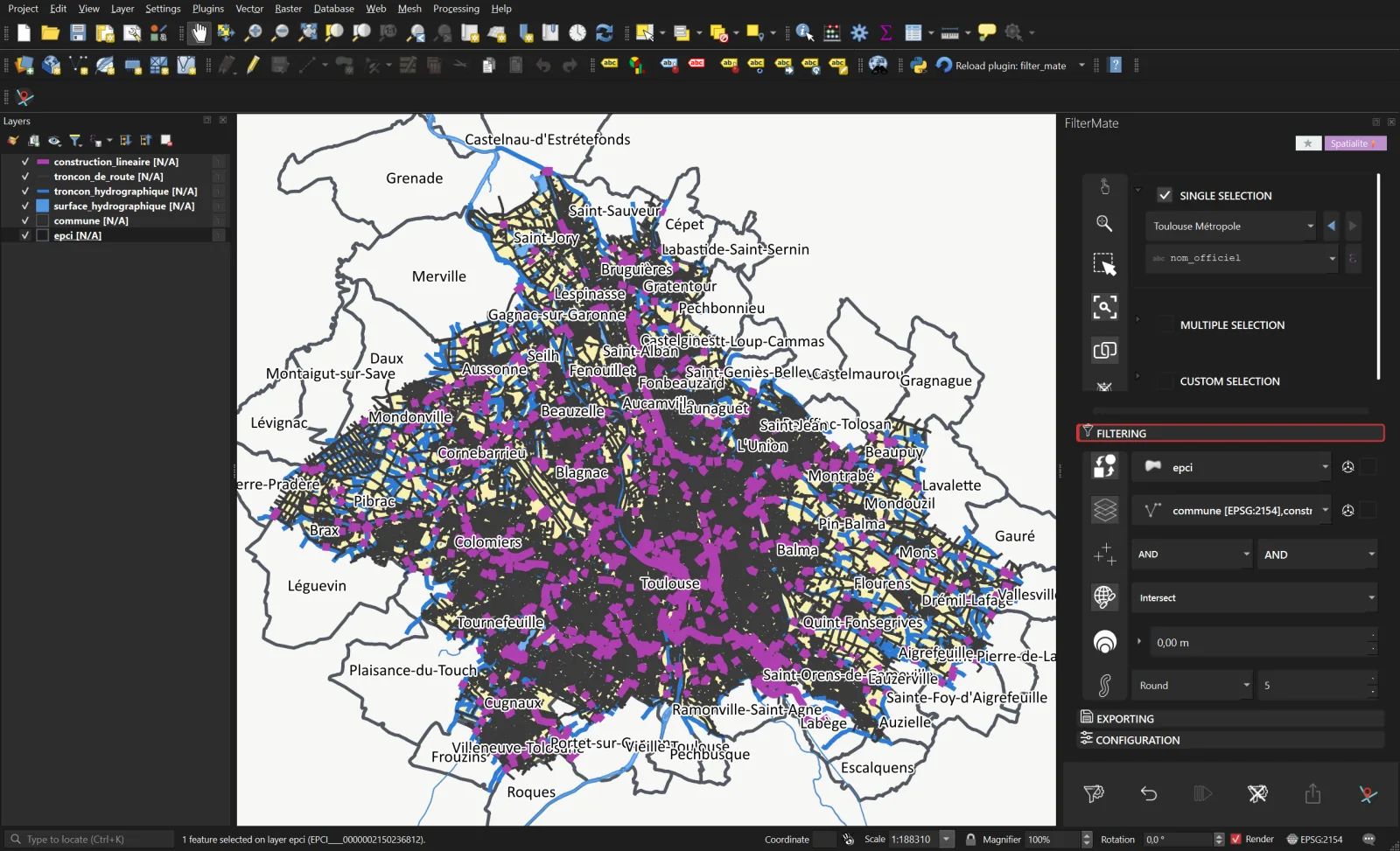
Step 1. The whole metropolis, Garonne, Hers and Touch included. - Keep only permanent watercourses. Source troncon_hydrographique, Custom selection
"persistance" = 'Permanent': 691 segments.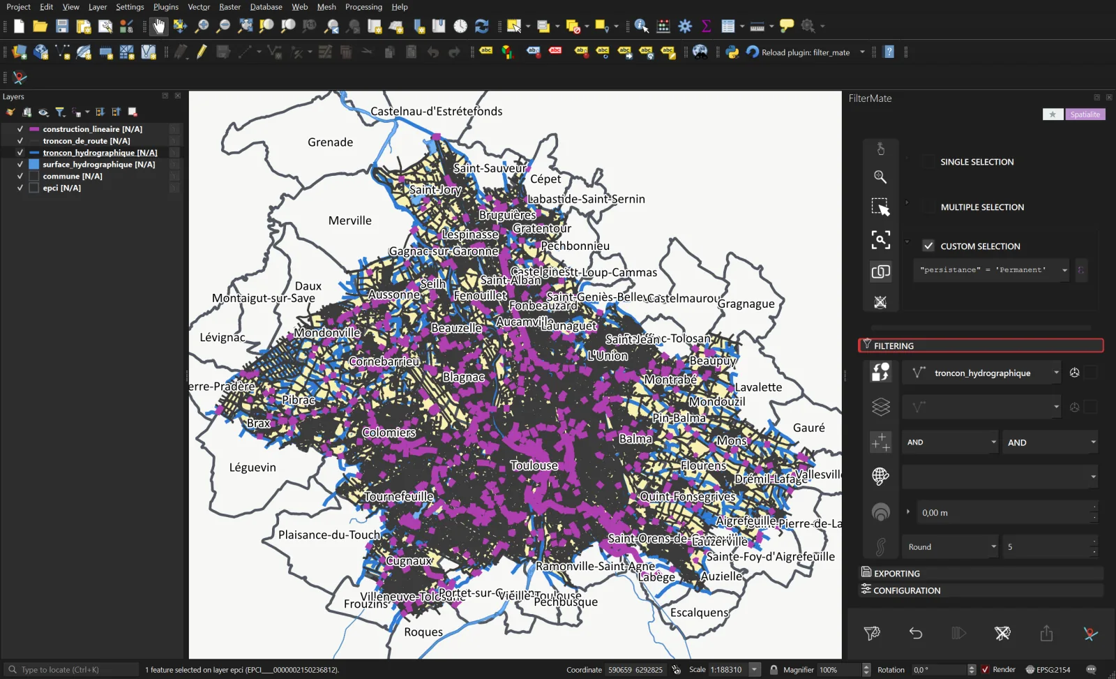
Step 2. Ditches and intermittent flows do not count. - Cross. Targets troncon_de_route and construction_lineaire, Cross predicate alone, Buffer row off. Filter.
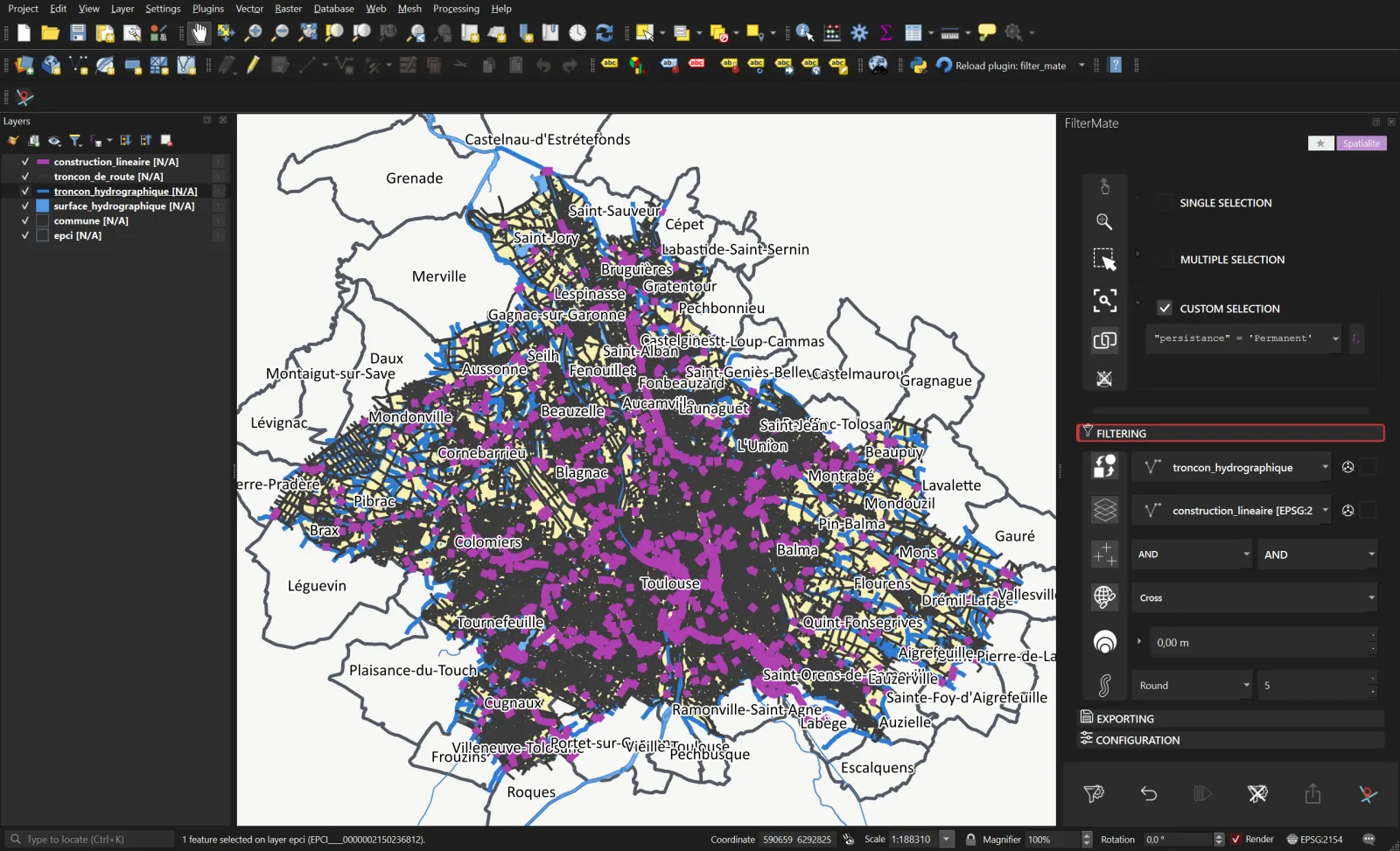
Step 3. One predicate, no buffer. 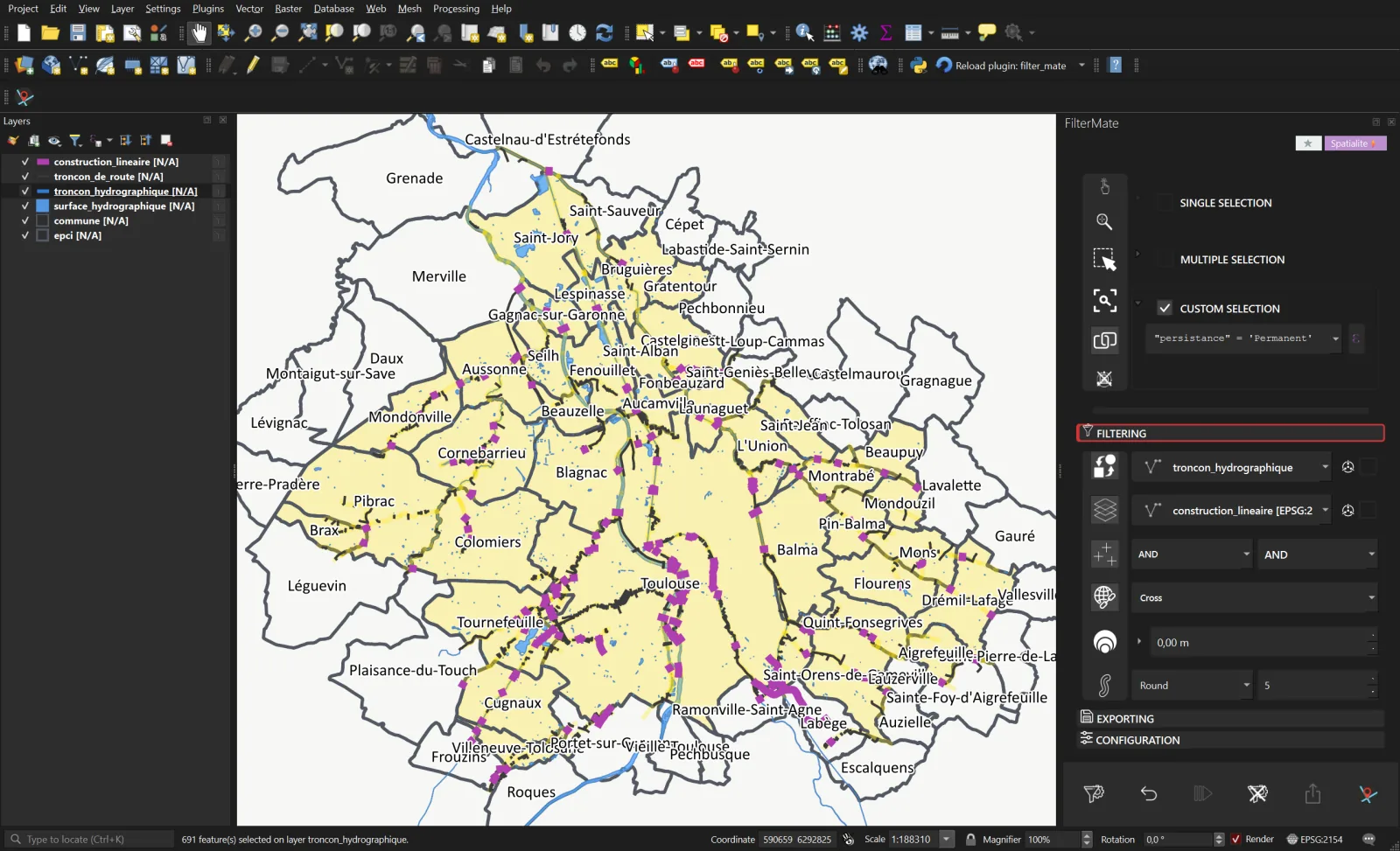
Result at metropolis scale: the crossings draw the river network. 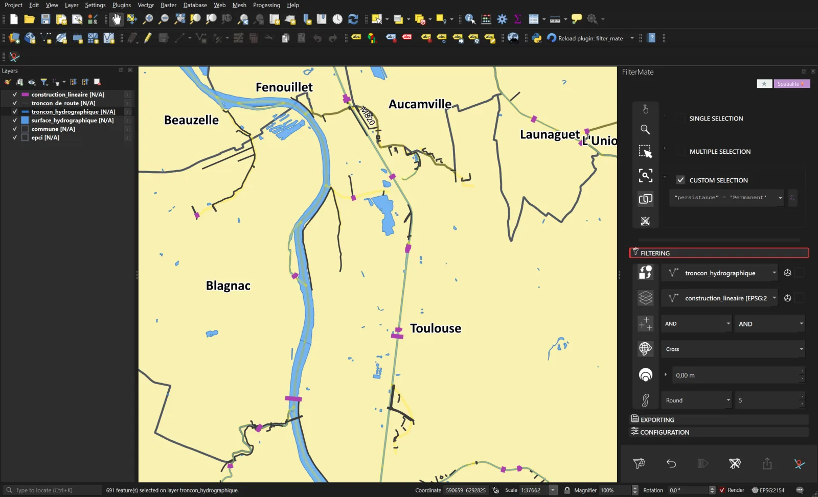
Zoom on the north of Toulouse: every remaining segment is a bridge or a crossing.
Result
1,112 road segments and 190 linear constructions (mostly bridges) cross a permanent watercourse within the metropolis extent.
5Clearing brush around homes
The need
Élodie, at the town hall of Bagnères-de-Luchon, must inform the owners subject to the legal brush-clearing obligation: vegetation within 50 m of a dwelling. She wants the map of the woods and forests concerned, without the hedges, which fall under another regime.
The FilterMate translation
Source batiment with the custom selection "usage_1" = 'Résidentiel', targets zone_de_vegetation and haie, Intersect, 50 m buffer. Then a second, attribute filter on the vegetation layer turned source, combined with AND with the previous spatial filter.
- Scope Luchon. 3,699 buildings, 269 vegetation zones, 123 hedges.
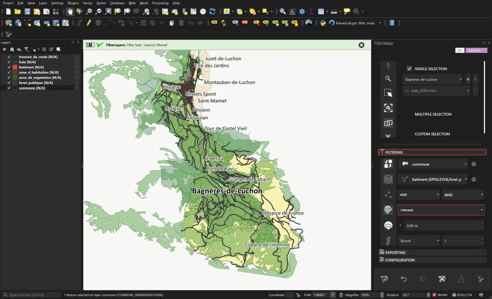
Step 1. The inhabited valley and the wooded slopes. - Keep only dwellings. Source batiment, Custom selection
"usage_1" = 'Résidentiel': 1,619 buildings.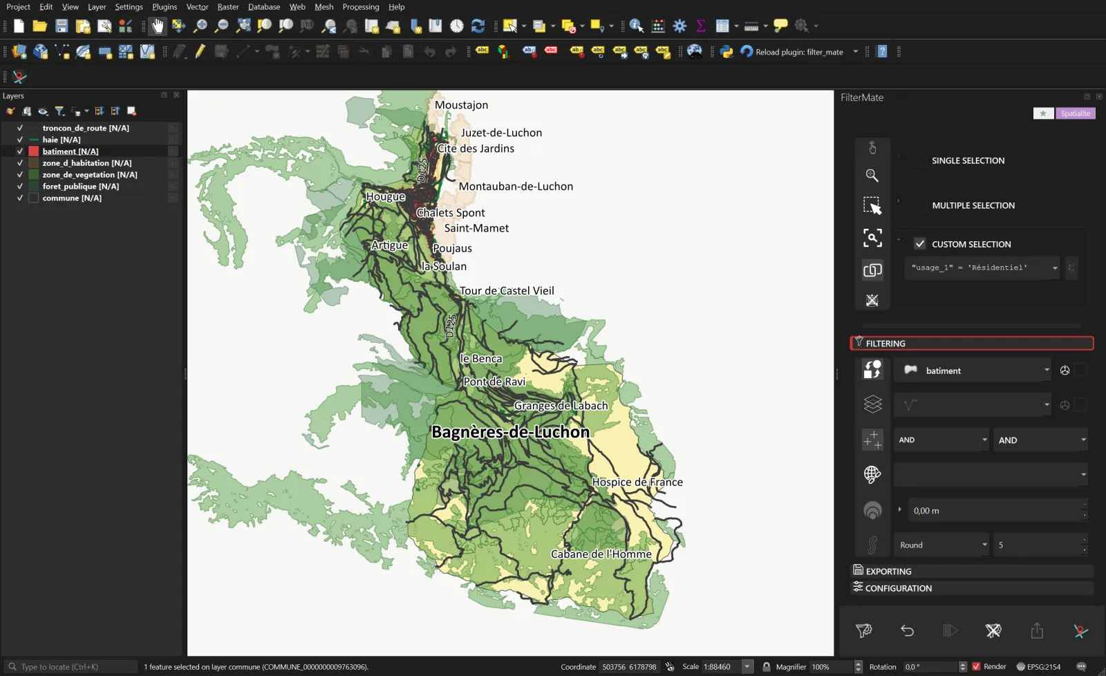
Step 2. Outbuildings, farm and industrial buildings are left out of the source. - 50 m. Targets zone_de_vegetation and haie, Intersect, Buffer 50. Filter: 119 vegetation zones and 48 hedges remain.
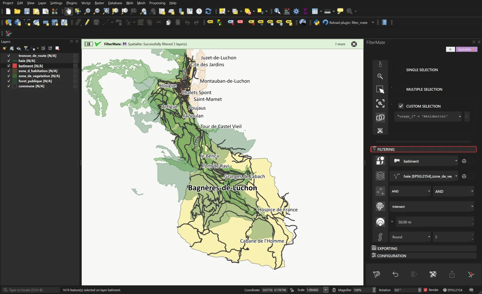
Step 3. Hedges and undifferentiated woods are still there. - Keep only woods and forests. Click zone_de_vegetation in the Layers panel: it becomes the source. Custom selection:
Enable the Combine operator row and leave AND on the left: the new filter narrows the spatial filter already applied to the source layer instead of replacing it."nature" IN ('Bois', 'Forêt fermée de feuillus', 'Forêt fermée de conifères', 'Forêt fermée mixte', 'Forêt ouverte')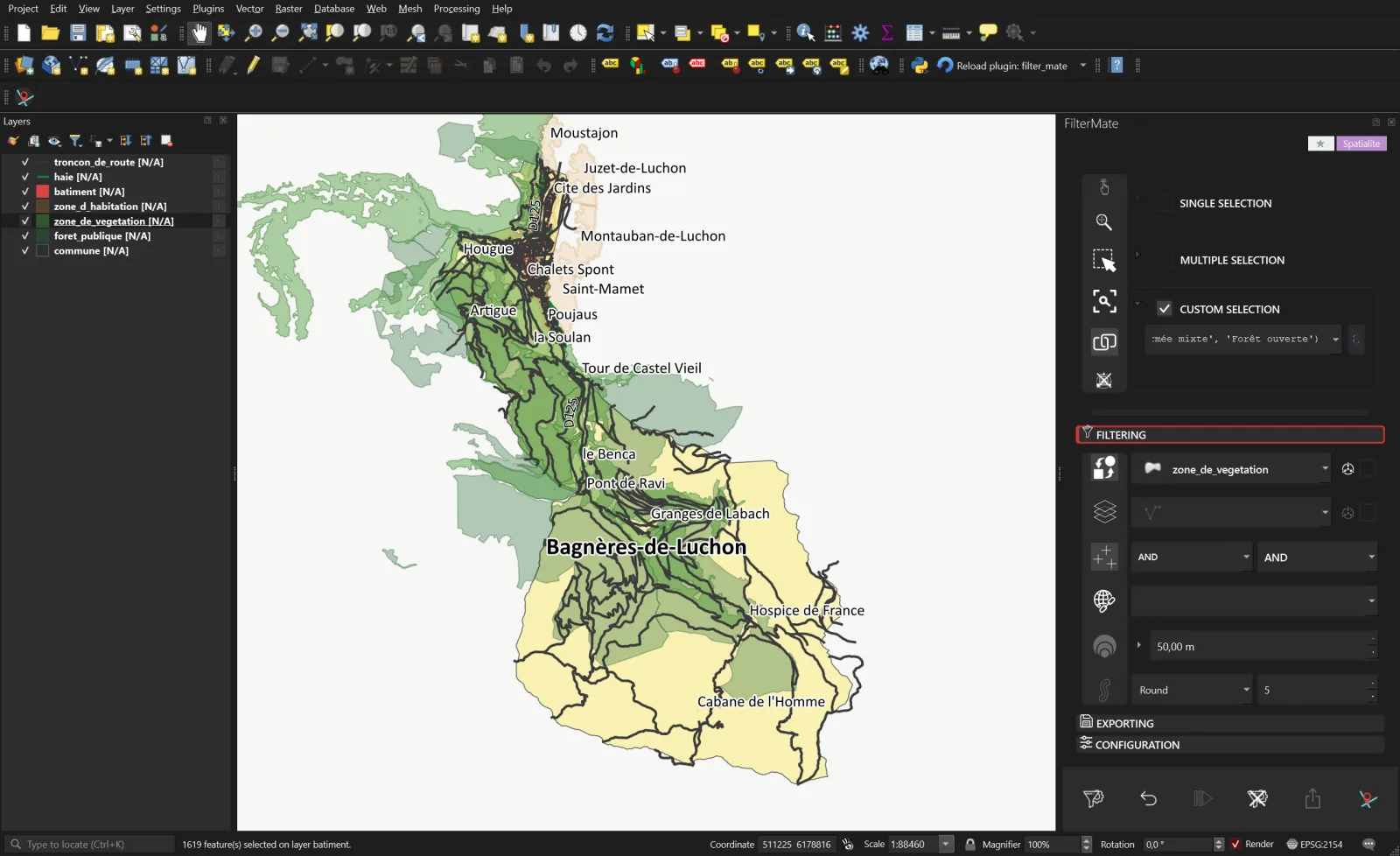
Step 4. The button of the Combine operator row is on, the left operator reads AND. - Filter.
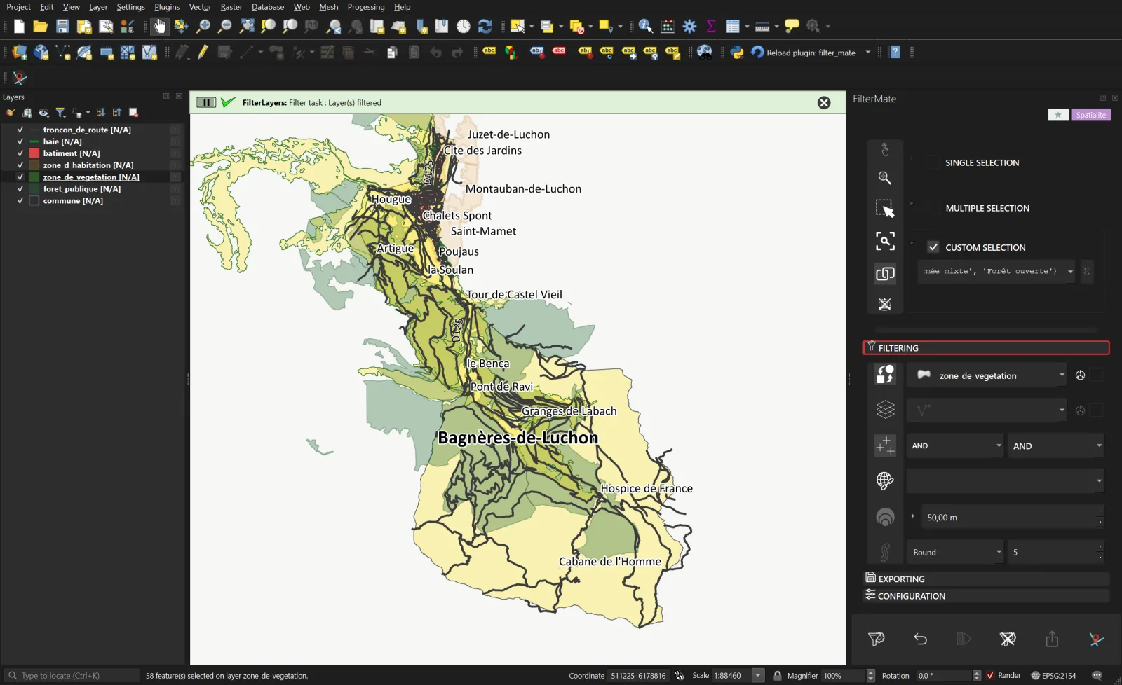
Step 5. 58 woods and forests within 50 m of a dwelling. 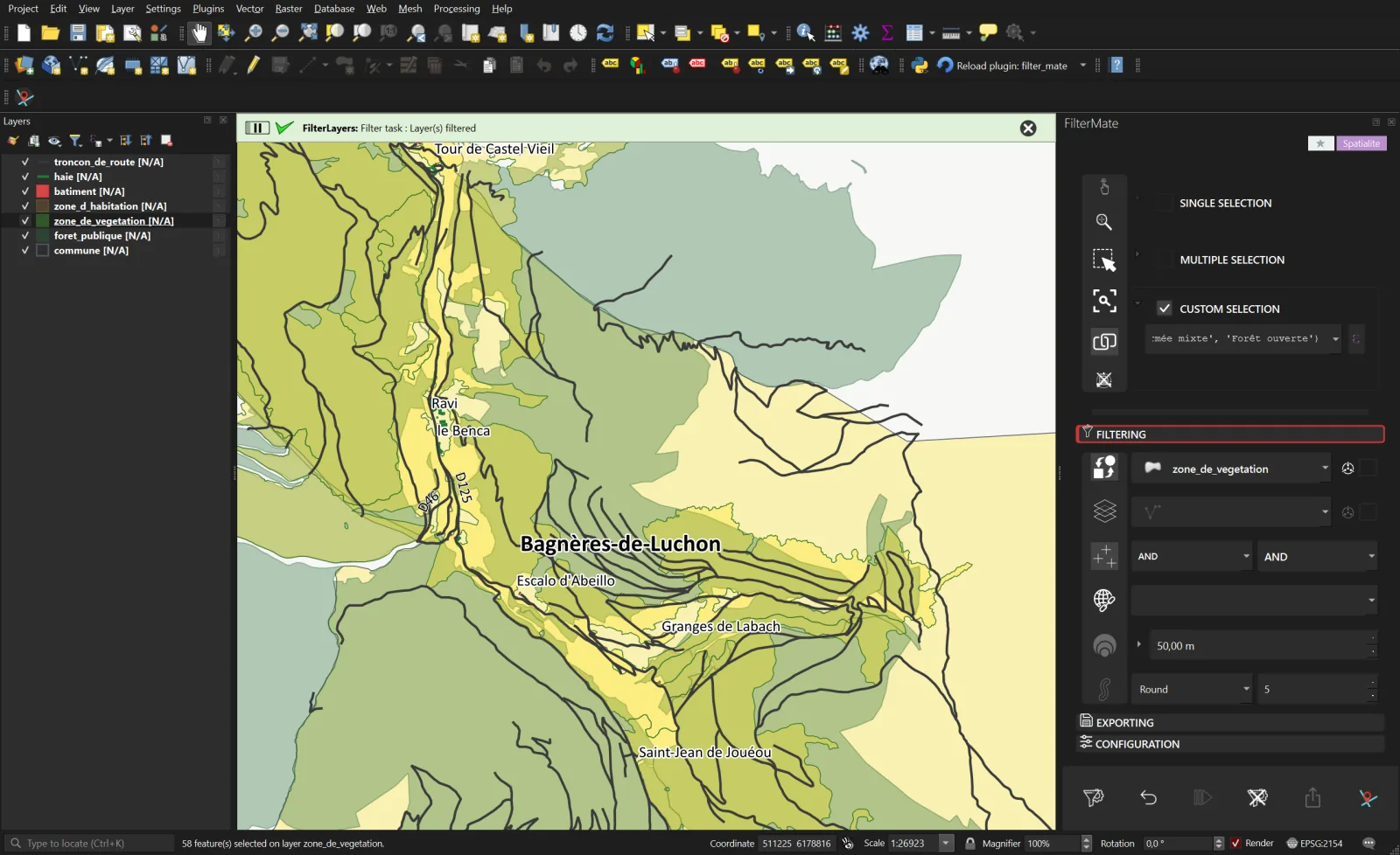
Zoom: the edges to clear surround the hillside neighbourhoods.
Result
Out of the commune's 269 vegetation zones, 119 touch the 50 m band around a dwelling, among which 58 woods and forests; 48 hedges are in the same case.
Under the hood
The vegetation layer's filter after step 5 keeps the spatial clause and adds the attribute clause:
(ROWID IN (SELECT id FROM "rtree_zone_de_vegetation_geometrie" WHERE …)
 AND ST_Intersects("geometrie", ST_Buffer(ST_MakeValid(ST_GeomFromText('MultiPolygon (…)', 2154)), 50.0)))
AND ("nature" IN ('Bois', 'Forêt fermée de feuillus', 'Forêt fermée de conifères', 'Forêt fermée mixte', 'Forêt ouverte'))6Hamlets the rescue services reach badly
The need
At the fire station of Aspet, in the Pyrenean foothills, the response plan is being prepared: which hamlets and activity zones lie more than 200 m from a paved road, hence reachable only by track or footpath?
The FilterMate translation
This is the Disjoint predicate with a 200 m buffer: keep what shares no point with the buffer zone. Since Disjoint keeps everything far away, including the rest of the department, the target layers are first scoped by an attribute filter on the INSEE code, applied with FilterMate's Processing algorithm. The second filter then combines with AND.
- Scope Aspet spatially for roads, buildings and vegetation (story 1), then by attribute for the two target layers: Toolbox → FilterMate → Filter multiple layers, layers zone_d_habitation and zone_d_activite_ou_d_interet, expression
"insee_commune" = '31020'. 87 hamlets and 31 activity zones.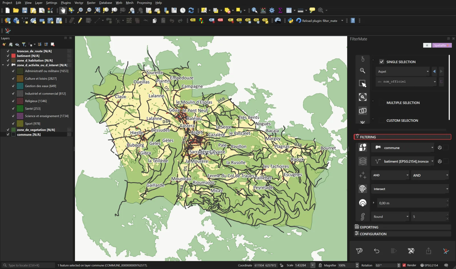
Step 1. The two target layers carry an attribute filter, the others a spatial one. - Keep only paved roads. Source troncon_de_route, Custom selection
"nature" NOT IN ('Chemin', 'Sentier', 'Escalier', 'Piste cyclable', 'Route empierrée'): 494 segments out of 1,168.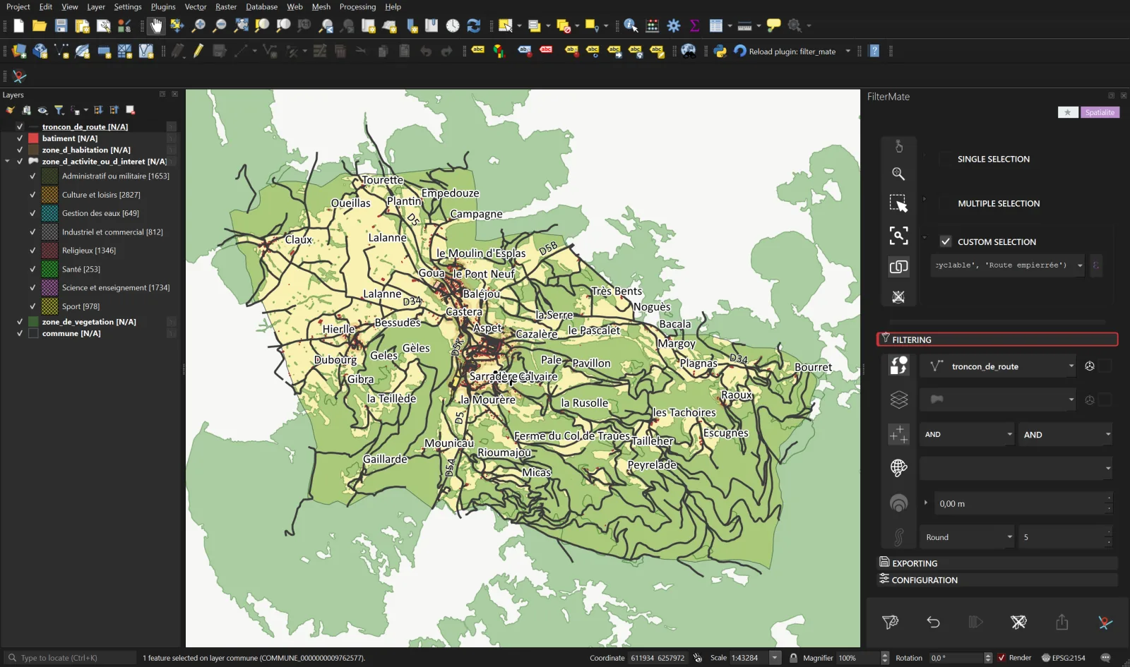
Step 2. Tracks and footpaths, plentiful in the mountains, are left out. - Disjoint, 200 m, AND. Targets zone_d_habitation and zone_d_activite_ou_d_interet, Disjoint predicate alone, Buffer 200, Combine operator row on with AND on the right (the target layers' operator).
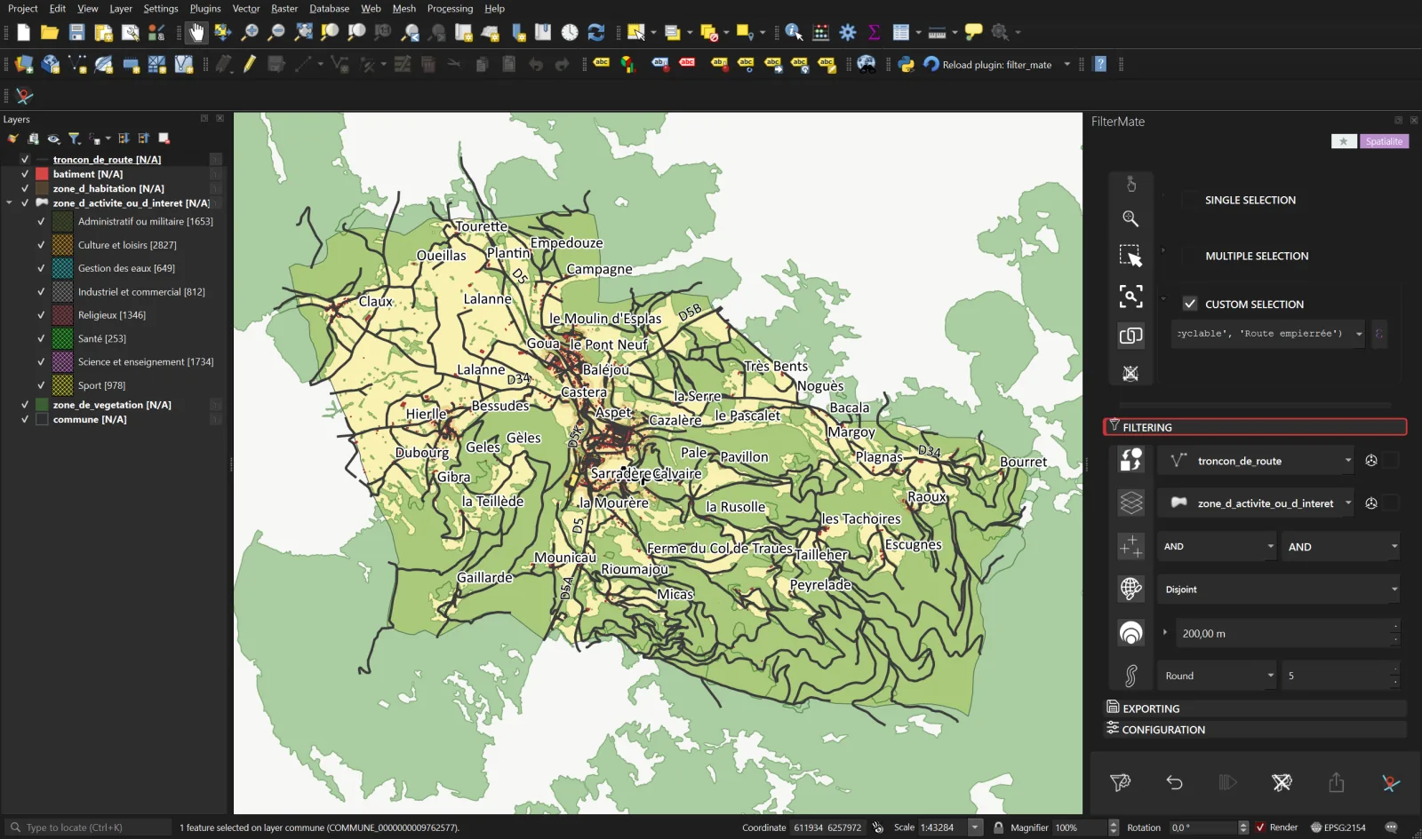
Step 3. Disjoint plus buffer: an exclusion ring. - Filter.
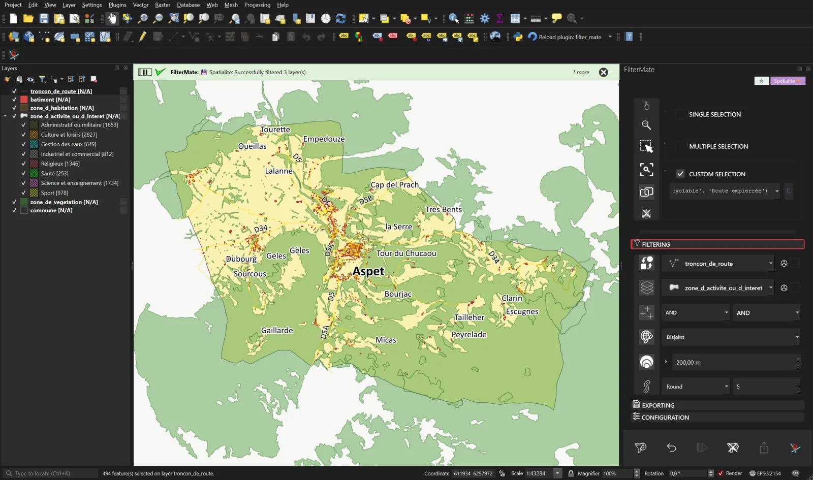
Step 4. The remaining hamlets are those no paved road comes within 200 m of.
Result
22 hamlets of Aspet are more than 200 m from a paved road; none of the 31 activity zones is. At 100 m they would be 32.
7The team's query library
The need
Julien (story 3) will redo the 300 m band at every BD TOPO update and wants his colleagues to replay it without him. The filter must exist outside his head: named, described, reapplicable in one click, exportable.
The FilterMate translation
A favorite records the complete filter: source layer, selection, predicates, buffer, target layers. The menu opens from the ★ badge in the header; the manager lets you rename, describe, change the scope (this project or all projects) and export as JSON. With the sharing extension, a shared git repository becomes the team library.
- Save. The 300 m filter of story 3 is applied. Click the ★ badge then Add filter, name it "PPRI Garonne 300 m".
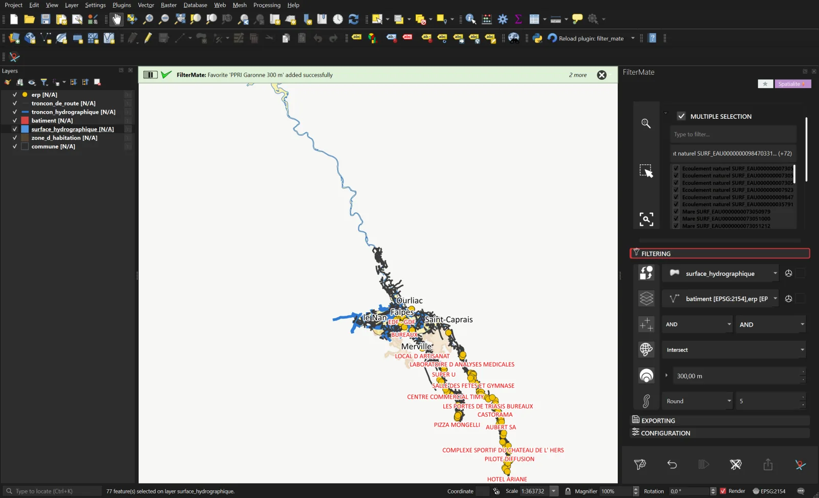
Step 1. The message bar confirms the save; the favorite immediately shows in the Quick filtering section of the ★ menu. - Unfilter. The three layers get the whole department back: 1,173,829 buildings.
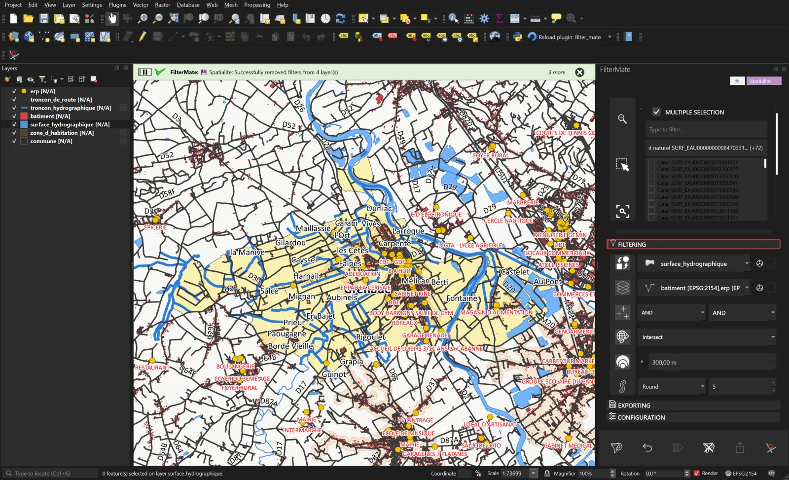
Step 2. Back to the unfiltered state. - Replay. ★ badge then "PPRI Garonne 300 m": the filter reapplies, with the same 14,181 buildings, 168 public buildings and 6,243 segments.
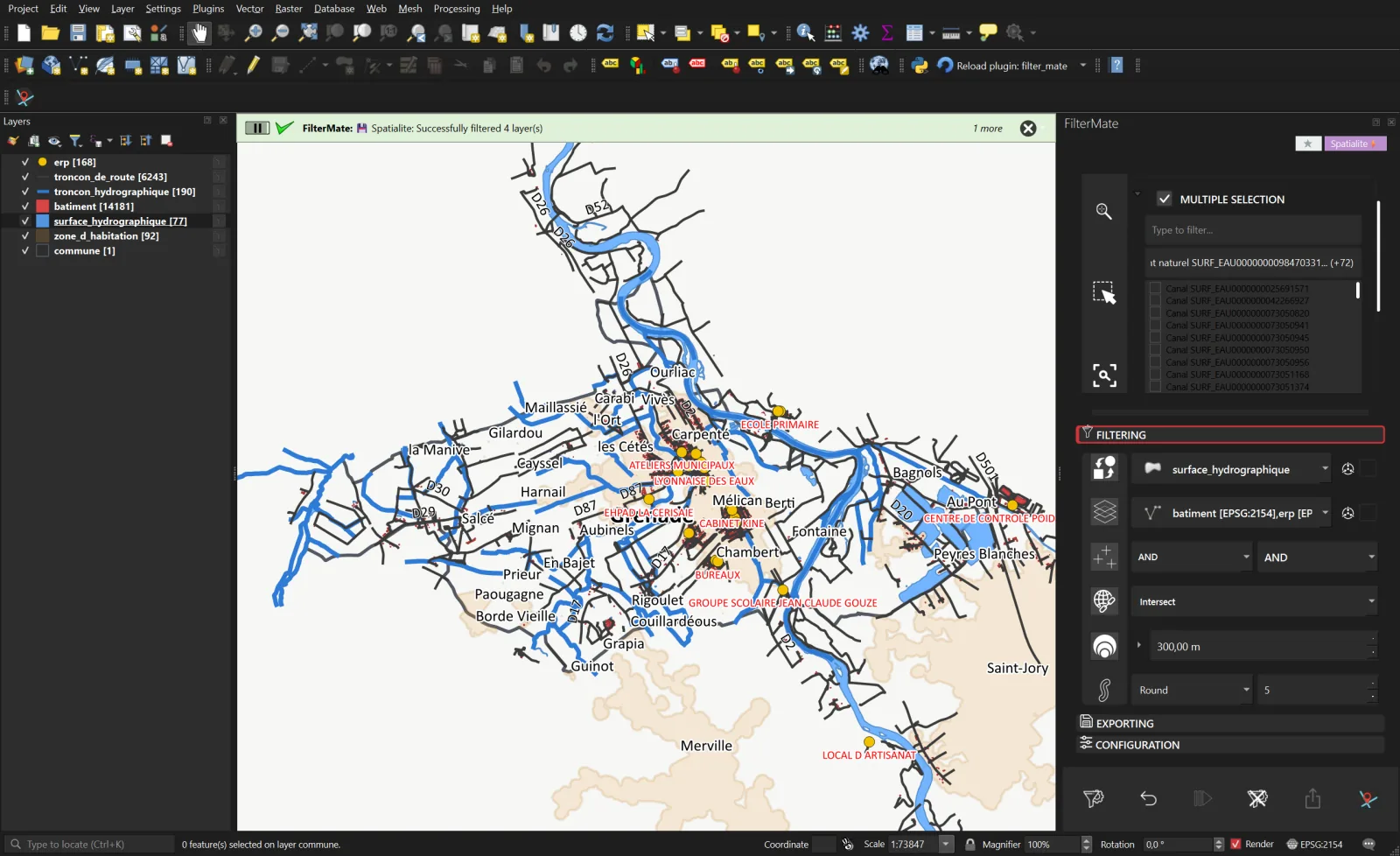
Step 3. Same result, one click. - Describe and share. Manage favorites… opens the manager: description, tags, scope, exact expression, Remote tab to publish to a git repository. Export… writes a JSON file to send to a colleague, who imports it from the same menu.
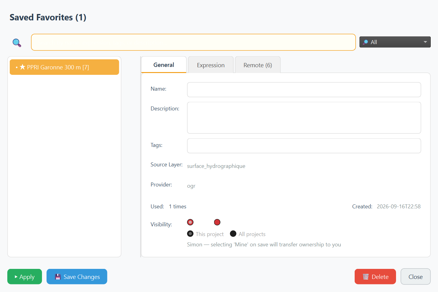
Step 4. The manager: list on the left, details and expression on the right.
8What changed since the last edition?
The need
Sophie administers the department's GIS and has just received the March 2026 edition of the BD TOPO. Before publishing it, she wants to isolate the objects modified since the previous edition on four layers, for a quality check, and be able to redo that check in a Processing model at every edition.
The FilterMate translation
No geometry here: a single attribute filter to apply to several layers. That is the job of the filtermate:batch_filter algorithm of the Processing toolbox, usable in the graphical modeler, in batch mode or from Python.
- Open the toolbox and search for "filtermate".
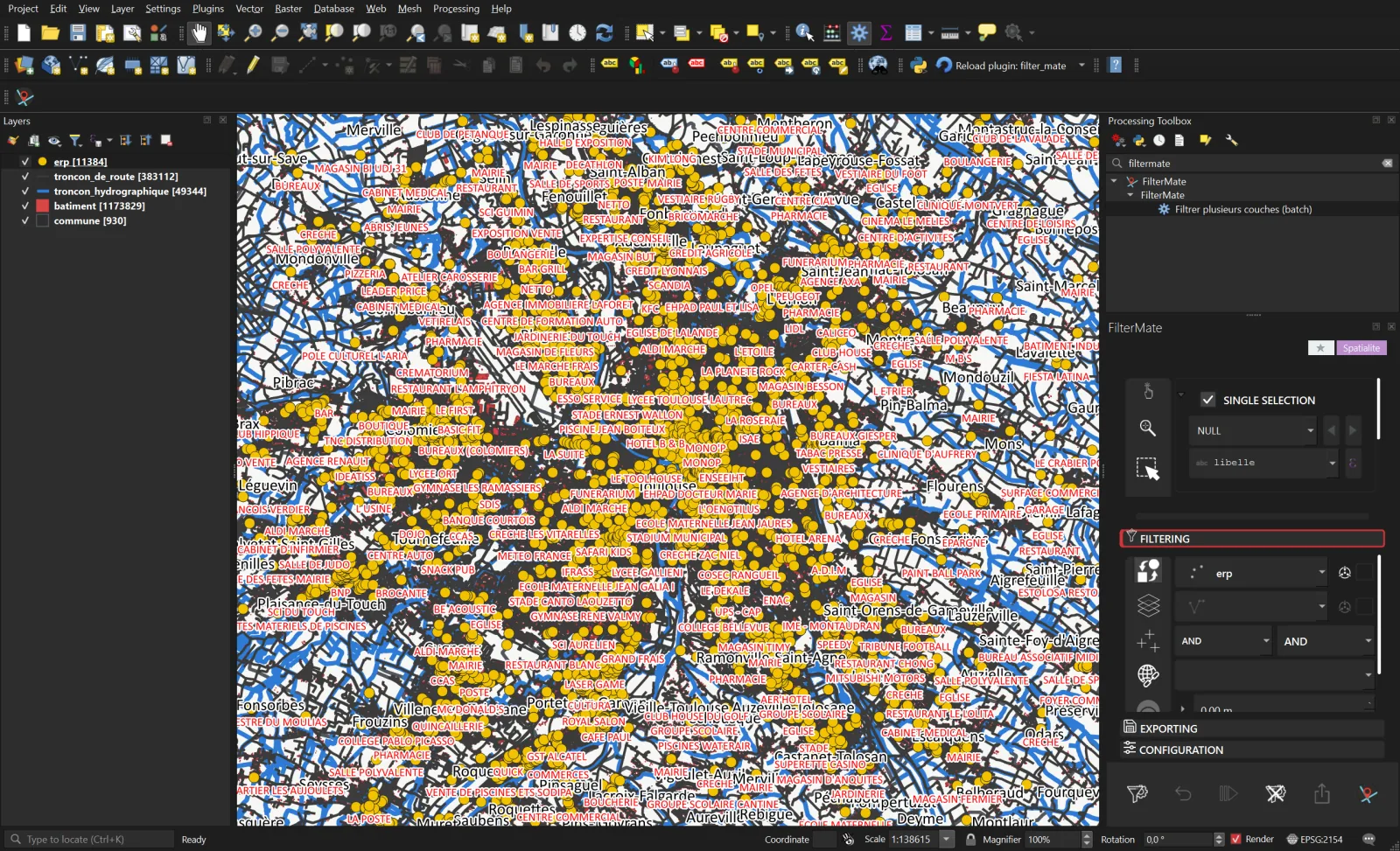
Step 1. The FilterMate provider and its batch filter algorithm. - Choose the layers and the expression. batiment, troncon_de_route, troncon_hydrographique, erp and the expression
"date_modification" >= '2025-03-15'.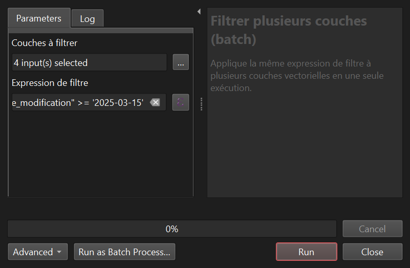
Step 2. An ordinary Processing dialog: it chains in a model like any other. - Run. The four layers receive the filter in one pass.
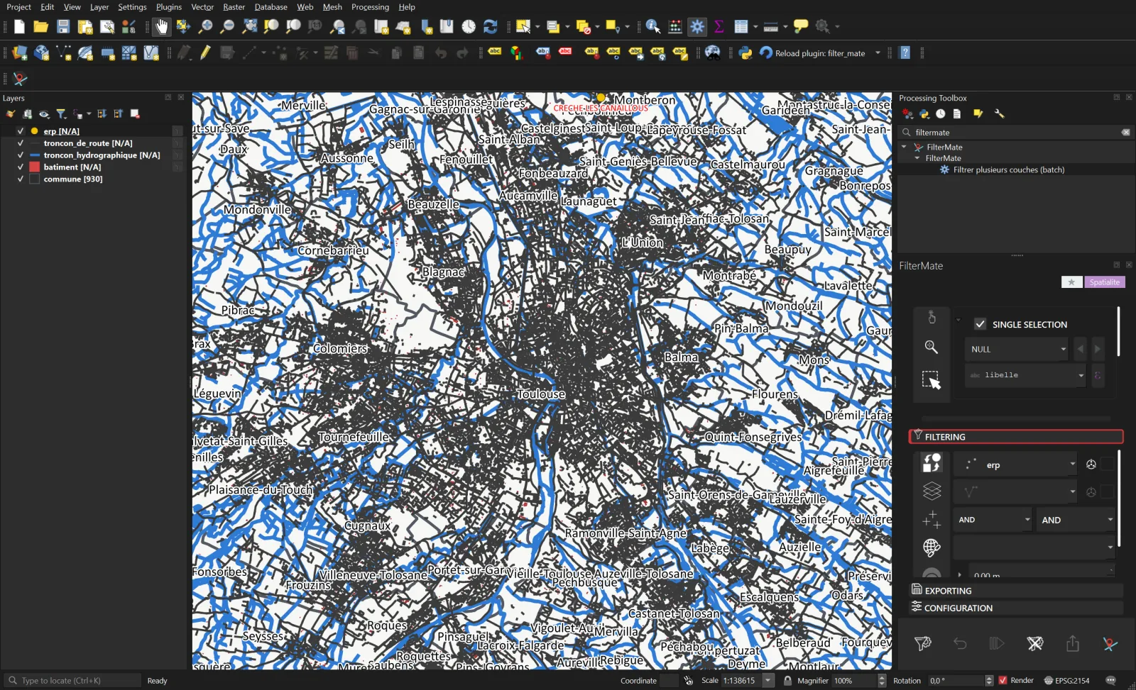
Step 3. Around Toulouse, the objects modified in the last year.
Result
| Layer | Department | Modified since 15 March 2025 |
|---|---|---|
| troncon_de_route | 383,112 | 173,616 |
| troncon_hydrographique | 49,344 | 28,519 |
| batiment | 1,173,829 | 22,954 |
| erp | 11,384 | 3 |
The same thing from the Python console
import processing
processing.run("filtermate:batch_filter", {
    "INPUT_LAYERS": ["batiment", "troncon_de_route", "troncon_hydrographique", "erp"],
    "EXPRESSION": "\"date_modification\" >= '2025-03-15'",
})9Replaying these stories at home
- Download the BD TOPO of your department from the IGN Géoplateforme ("all themes", GeoPackage format, Lambert-93). The file ships with its spatial indexes: that is what makes the cascades fast.
- Load the layers named in each story. The styles embedded in the GeoPackage hide buildings beyond 1:25,000: disable scale-dependent visibility in the layer properties, or apply your own styles.
- Replace the commune names with yours. The fields used (
nom_officiel,importance,persistance,usage_1,nature,insee_commune,date_modification) are those of BD TOPO 3.x, identical in every department. - To reproduce the screenshots, the repository script
scripts/recipe_screenshots.pydrives QGIS from end to end of each story, checks the counts and saves one image per step.